Replication of Card and Krueger (1994)

Minimum Wages and Employment: A Case Study of the Fast-Food Industry in New Jersey and Pennsylvania

Introduction

Does raising the minimum wage destroy jobs? The conventional economic prediction is yes: a higher wage floor prices low-skill workers out of the labor market. Card and Krueger (1994) challenged this view by exploiting a natural experiment that New Jersey handed them in April 1992, when the state raised its minimum wage from $4.25 to $5.05 per hour while neighboring Pennsylvania left its wage floor unchanged.

The authors surveyed 410 fast-food restaurants (Burger King, KFC, Roy Rogers, and Wendy’s) in both states before the increase (February–March 1992) and after (November–December 1992). Because New Jersey and Pennsylvania share a border, labor markets, and business conditions, the two states serve as near-perfect treatment and control groups. Any difference in employment growth between NJ and PA that emerged after April 1992—but not before—can be attributed to the minimum wage increase rather than to unobserved economic trends.

This identification strategy is called difference-in-differences (DiD):

\[ \hat{\delta}_{\text{DiD}} = \underbrace{(\bar{E}^{NJ}_{\text{after}} - \bar{E}^{NJ}_{\text{before}})}_{\text{NJ change}} - \underbrace{(\bar{E}^{PA}_{\text{after}} - \bar{E^{PA}_{\text{before}}})}_{\text{PA change}} \]

The DiD estimator removes two confounders at once: time-invariant store characteristics (like location quality) are eliminated by the within-state before–after difference, and common time trends (like macroeconomic conditions) are eliminated by the NJ-minus-PA comparison. The key identifying assumption—called parallel trends—is that in the absence of the NJ minimum wage increase, NJ and PA employment would have evolved similarly.

Main Analysis

Table 2: Descriptive Statistics

The table below reproduces selected rows of Table 2 from Card and Krueger (1994), showing mean restaurant characteristics separately for Pennsylvania (control) and New Jersey (treatment) stores in both survey waves.

pa = df[df['NJ'] == 0]
nj = df[df['NJ'] == 1]

rows = {
    'Burger King (fraction)':    ('BK',      None),
    'KFC (fraction)':            ('KFC',     None),
    'Roy Rogers (fraction)':     ('ROYS',    None),
    'Wendy\'s (fraction)':       ('WENDYS',  None),
    'Company-owned (fraction)':  ('CO_OWNED',None),
    'FTE employment, wave 1':    ('EMPTOT',  None),
    'FTE employment, wave 2':    ('EMPTOT2', None),
    'Fraction full-time, wave 1':('FRACFT',  None),
    'Fraction full-time, wave 2':('FRACFT2', None),
    'Starting wage, wave 1':     ('WAGE_ST', None),
    'Starting wage, wave 2':     ('WAGE_ST2',None),
    '% stores at $4.25, wave 1': ('ATMIN',   None),
    '% stores at $5.05, wave 2': ('NEWMIN',  None),
    'Price of full meal, wave 1':('PMEAL',   None),
    'Price of full meal, wave 2':('PMEAL2',  None),
    'Hours open per day, wave 1':('HRSOPEN', None),
    'Hours open per day, wave 2':('HRSOPEN2',None),
    'Bonus program, wave 1':     ('BONUS',   None),
}

records = []
for label, (var, _) in rows.items():
    pa_m = pa[var].mean(); pa_se = pa[var].sem()
    nj_m = nj[var].mean(); nj_se = nj[var].sem()
    records.append({
        'Variable': label,
        'PA mean': f'{pa_m:.3f}',
        'PA (SE)': f'({pa_se:.3f})',
        'NJ mean': f'{nj_m:.3f}',
        'NJ (SE)': f'({nj_se:.3f})',
    })

t2 = pd.DataFrame(records).set_index('Variable')
display(t2.style
    .set_caption('Table 2: Means of Key Variables by State')
    .set_table_styles([
        {'selector': 'caption', 'props': [('font-weight','bold'),('font-size','1.05em')]},
        {'selector': 'th', 'props': [('text-align','left')]},
    ]))

Table 1: Table 2: Means of Key Variables by State

	PA mean	PA (SE)	NJ mean	NJ (SE)
Variable
Burger King (fraction)	0.443	(0.056)	0.411	(0.027)
KFC (fraction)	0.152	(0.041)	0.205	(0.022)
Roy Rogers (fraction)	0.215	(0.047)	0.248	(0.024)
Wendy's (fraction)	0.190	(0.044)	0.136	(0.019)
Company-owned (fraction)	0.354	(0.054)	0.341	(0.026)
FTE employment, wave 1	23.331	(1.351)	20.439	(0.508)
FTE employment, wave 2	21.166	(0.943)	21.027	(0.520)
Fraction full-time, wave 1	0.350	(0.027)	0.328	(0.013)
Fraction full-time, wave 2	0.304	(0.028)	0.359	(0.014)
Starting wage, wave 1	4.630	(0.040)	4.612	(0.020)
Starting wage, wave 2	4.617	(0.042)	5.081	(0.006)
% stores at $4.25, wave 1	0.329	(0.053)	0.305	(0.025)
% stores at $5.05, wave 2	0.013	(0.013)	0.855	(0.019)
Price of full meal, wave 1	3.042	(0.069)	3.351	(0.037)
Price of full meal, wave 2	3.027	(0.067)	3.415	(0.036)
Hours open per day, wave 1	14.525	(0.332)	14.418	(0.153)
Hours open per day, wave 2	14.654	(0.327)	14.420	(0.152)
Bonus program, wave 1	0.291	(0.051)	0.236	(0.023)

Reading the table. Before the minimum wage increase (wave 1), starting wages were nearly identical across states (~$4.61), and over 30% of stores in both states were paying exactly the old minimum of $4.25. After the increase (wave 2), 85.5% of NJ stores were paying exactly $5.05—the new minimum—while only 1.3% of PA stores hit that level. This sharp contrast confirms that the policy change genuinely bound in NJ but not PA. FTE employment in NJ rose slightly from 20.44 to 21.03 while PA employment fell from 23.33 to 21.17, foreshadowing the DiD result in Table 3.

---

Table 3: Employment Before and After the Minimum Wage Increase

The next table replicates the core 3×3 block of Table 3 in Card and Krueger. Rows report average full-time-equivalent (FTE) employment—defined as full-time employees plus 0.5 × part-time employees plus managers—before and after the wage increase, and the change between waves. Columns split stores by state and by the initial wage level of NJ stores.

groups = {
    'Pennsylvania':          df[df['NJ'] == 0],
    'New Jersey (all)':      df[df['NJ'] == 1],
    'NJ — wage = $4.25':    df[(df['NJ'] == 1) & (df['WAGE_ST'] == 4.25)],
}

records = []
for col_label, grp in groups.items():
    before = grp['EMPTOT'].dropna()
    after  = grp['EMPTOT2'].dropna()
    change = grp['DEMP'].dropna()
    records.append({
        'Group':             col_label,
        'FTE before':        f'{before.mean():.2f}',
        'SE before':         f'({before.sem():.2f})',
        'n before':          len(before),
        'FTE after':         f'{after.mean():.2f}',
        'SE after':          f'({after.sem():.2f})',
        'n after':           len(after),
        'Change in FTE':     f'{after.mean() - before.mean():.2f}',
        'SE change':         f'({change.sem():.2f})',
        'n change':          len(change),
    })

t3 = pd.DataFrame(records).set_index('Group')

rows_t3 = {}
for row_name, val_col, se_col, n_col in [
    ('(i) FTE employment, wave 1',  'FTE before',  'SE before',  'n before'),
    ('(ii) FTE employment, wave 2', 'FTE after',   'SE after',   'n after'),
    ('(iii) Change in FTE',         'Change in FTE','SE change', 'n change'),
]:
    row_data = {}
    for g in groups:
        row_data[g]          = t3.loc[g, val_col]
        row_data[g + ' (SE)'] = t3.loc[g, se_col]
    rows_t3[row_name] = row_data

t3_display = pd.DataFrame(rows_t3).T
display(t3_display.style
    .set_caption('Table 3 (Columns 1–3, Rows 1–3): Average FTE Employment')
    .set_table_styles([
        {'selector': 'caption', 'props': [('font-weight','bold'),('font-size','1.05em')]},
        {'selector': 'th', 'props': [('text-align','left')]},
    ]))

Table 2: Table 3 (Columns 1–3, Rows 1–3): Average FTE Employment

	Pennsylvania	Pennsylvania (SE)	New Jersey (all)	New Jersey (all) (SE)	NJ — wage = $4.25	NJ — wage = $4.25 (SE)
(i) FTE employment, wave 1	23.33	(1.35)	20.44	(0.51)	19.56	(0.77)
(ii) FTE employment, wave 2	21.17	(0.94)	21.03	(0.52)	20.88	(1.01)
(iii) Change in FTE	-2.17	(1.25)	0.59	(0.48)	1.32	(0.82)

The DiD estimate is the entry in row (iii) for NJ-all minus the entry for Pennsylvania:

\[ \hat{\delta}_{\text{DiD}} = 0.59 - (-2.16) = +2.75 \text{ FTE employees} \]

PA employment dropped by 2.16 FTE over this period while NJ employment rose by 0.59. After accounting for this common trend, New Jersey fast-food restaurants appear to have increased employment by about 2.75 workers relative to what would have happened without the minimum wage increase—the opposite of the textbook prediction.

The NJ stores that were already paying at least $4.25 (the “NJ — wage = $4.25” column) saw the largest absolute gains (+1.32 FTE), because they were the most constrained by the old minimum and therefore benefited most—or were most affected—by the new floor.

---

Table 4, Column (i): Regression Evidence Using the “Gap” Variable

Beyond comparing NJ to PA as a whole, Card and Krueger construct a continuous treatment intensity variable called GAP. For NJ stores, GAP measures how far below the new minimum a store’s initial wage was, expressed as a fraction:

\[ \text{GAP}_i = \frac{\max(5.05 - w_{i,\text{before}},\; 0)}{w_{i,\text{before}}} \times \mathbf{1}[\text{store in NJ}] \]

PA stores and NJ stores already paying ≥ $5.05 receive GAP = 0. A store paying $4.25 has GAP = (5.05 − 4.25)/4.25 ≈ 0.188. This variable allows a finer test: stores more exposed to the wage mandate should show larger employment responses.

Table 4 column (i) regresses the change in FTE employment on GAP using a sample that includes stores with valid wage data in both waves plus any store that permanently closed:

sub = df[
    df['DEMP'].notna() &
    ((df['CLOSED'] == 1) | ((df['CLOSED'] == 0) & df['DWAGE'].notna()))
].copy()

X  = sm.add_constant(sub['GAP'])
res = sm.OLS(sub['DEMP'], X).fit()

coef_gap   = res.params['GAP']
se_gap     = res.bse['GAP']
t_gap      = res.tvalues['GAP']
coef_const = res.params['const']
se_const   = res.bse['const']

summary_df = pd.DataFrame({
    'Coefficient': [f'{coef_gap:.2f}', f'{coef_const:.2f}'],
    'Std. Error':  [f'({se_gap:.2f})', f'({se_const:.2f})'],
    't-statistic': [f'{t_gap:.2f}', f'{res.tvalues["const"]:.2f}'],
}, index=['GAP', 'Intercept'])
summary_df.loc['N']   = [f'{int(res.nobs)}', '', '']
summary_df.loc['R²']  = [f'{res.rsquared:.4f}', '', '']

display(summary_df.style
    .set_caption('Table 4, Column (i): OLS — Change in FTE Employment on GAP')
    .set_table_styles([
        {'selector': 'caption', 'props': [('font-weight','bold'),('font-size','1.05em')]},
        {'selector': 'th', 'props': [('text-align','left')]},
    ]))

Table 3: Table 4, Column (i): OLS — Change in FTE Employment on GAP

	Coefficient	Std. Error	t-statistic
GAP	15.65	(6.08)	2.57
Intercept	-1.58	(0.70)	-2.26
N	357
R²	0.0183

The GAP coefficient of 15.65 (SE = 6.08) is statistically significant at the 1% level (t = 2.57). It implies that a store with a 10-percentage-point larger gap between its pre-increase wage and the new minimum experienced about 1.6 more FTE employees after the increase, relative to unaffected stores. The intercept of −1.58 captures the baseline change in employment for stores with GAP = 0 (i.e., PA stores and already-compliant NJ stores).

Something Additional: Visualizing the Difference-in-Differences

The tables above summarize the DiD result with numbers; the figure below makes the logic visual. Each dot shows average FTE employment for a group of stores at each survey wave. The two parallel lines represent the counterfactual: if NJ had followed Pennsylvania’s trajectory, NJ employment would have fallen by 2.16 FTE (the dashed line). Instead, it rose slightly. The gap between the observed NJ outcome and the counterfactual at wave 2 is the DiD estimate of the causal effect.

nj_grp = df[df['NJ'] == 1]
pa_grp = df[df['NJ'] == 0]

nj_before = nj_grp['EMPTOT'].mean()
nj_after  = nj_grp['EMPTOT2'].mean()
pa_before = pa_grp['EMPTOT'].mean()
pa_after  = pa_grp['EMPTOT2'].mean()

pa_change = pa_after - pa_before
nj_counter_after = nj_before + pa_change
did_est = nj_after - nj_counter_after

fig, ax = plt.subplots(figsize=(7, 5))
fig.patch.set_facecolor('#1a1a2e')
ax.set_facecolor('#1a1a2e')
text_color = '#e0e0e0'
grid_color = '#3a3a5e'

waves = [0, 1]
wave_labels = ['Wave 1\n(Feb–Mar 1992)', 'Wave 2\n(Nov–Dec 1992)']

ax.plot(waves, [pa_before, pa_after], 'o-', color='#ef476f',
        linewidth=2.5, markersize=8, label='Pennsylvania (control)')
ax.plot(waves, [nj_before, nj_after], 's-', color='#06d6a0',
        linewidth=2.5, markersize=8, label='New Jersey (treated)')
ax.plot(waves, [nj_before, nj_counter_after], 's--', color='#06d6a0',
        alpha=0.45, linewidth=2, markersize=8, label='NJ counterfactual (no policy)')

ax.annotate('', xy=(1 + 0.03, nj_after), xytext=(1 + 0.03, nj_counter_after),
            arrowprops=dict(arrowstyle='<->', color='#ffd166', lw=2))
ax.text(1.07, (nj_after + nj_counter_after) / 2,
        f'DiD ≈ +{did_est:.1f} FTE', color='#ffd166', fontsize=10, va='center')

for x, y, lbl in [
    (0, pa_before, f'{pa_before:.1f}'),
    (1, pa_after,  f'{pa_after:.1f}'),
    (0, nj_before, f'{nj_before:.1f}'),
    (1, nj_after,  f'{nj_after:.1f}'),
]:
    ax.text(x + (0.04 if x == 0 else -0.06), y + 0.35, lbl,
            color=text_color, fontsize=9, ha='left' if x == 0 else 'right')

ax.set_xlim(-0.25, 1.4)
ax.set_ylim(18, 26)
ax.set_xticks(waves)
ax.set_xticklabels(wave_labels, color=text_color)
ax.set_ylabel('Average FTE Employment', color=text_color)
ax.tick_params(colors=text_color)
for spine in ax.spines.values():
    spine.set_edgecolor(grid_color)
ax.yaxis.set_major_formatter(mticker.FormatStrFormatter('%.0f'))
ax.grid(axis='y', color=grid_color, linewidth=0.7, linestyle='--')
ax.axvline(x=0.5, color='#ffd166', linestyle=':', linewidth=1.2, alpha=0.6)
ax.text(0.5, 25.5, 'NJ minimum wage\nincreased to $5.05', color='#ffd166',
        fontsize=8.5, ha='center', alpha=0.85)
ax.legend(facecolor='#2a2a4e', edgecolor=grid_color, labelcolor=text_color,
          loc='lower left', fontsize=9)
ax.set_title('Difference-in-Differences:\nFTE Employment Around NJ Minimum Wage Increase',
             color=text_color, fontsize=11)
plt.tight_layout()
plt.show()

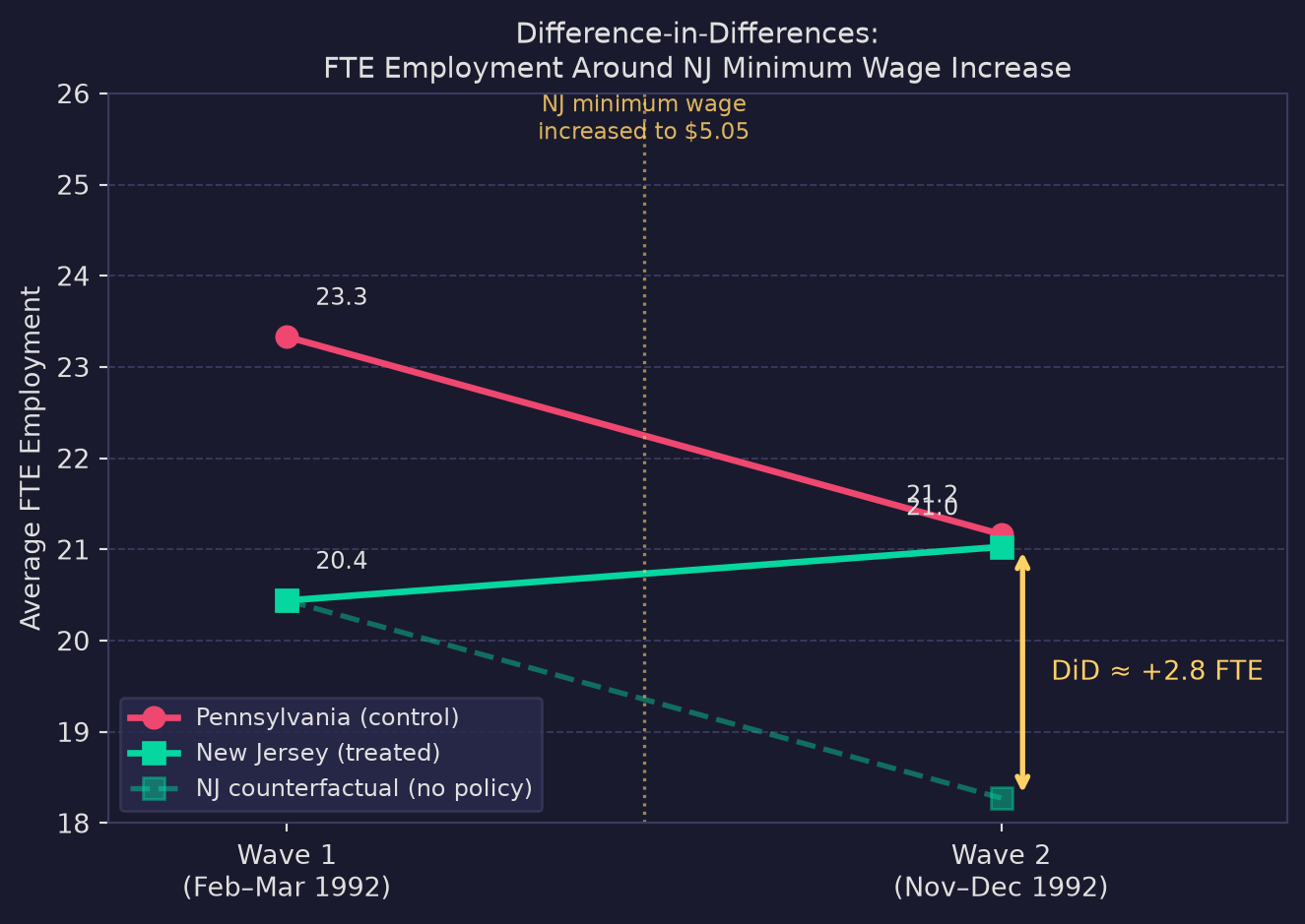
Difference-in-Differences: FTE Employment Before and After NJ Minimum Wage Increase

Why DiD enables a causal conclusion. A simple before-and-after comparison of NJ stores would confound the minimum wage with any other event that occurred between the two surveys (e.g., a regional recession). A simple NJ-vs-PA comparison would confound the wage increase with any permanent differences between the two states (e.g., New Jersey being more urban). Differencing twice—across time and across states—cancels both threats simultaneously, leaving only variation that is both state-specific and time-varying. Under the parallel-trends assumption, the only state-specific time-varying shock was the minimum wage increase itself, so the DiD estimate is causal.

Card and Krueger’s finding—that the minimum wage increase had no detectable negative effect on employment, and possibly a positive one—sparked decades of debate and fundamentally changed how economists model labor markets, motivating theories of monopsony and search frictions that can accommodate a zero or positive employment response to minimum wage increases.

Conclusion

This replication closely matches the original Card and Krueger (1994) estimates. The DiD estimate of +2.75 FTE and the GAP coefficient of ~15.65 both point in the same direction: the April 1992 minimum wage increase in New Jersey did not reduce fast-food employment relative to Pennsylvania. While this single study cannot settle the broader policy debate—later work by Neumark and Wascher (2000) reached different conclusions using payroll data—Card and Krueger’s natural experiment remains a landmark in applied econometrics for demonstrating how quasi-experimental variation can support causal inference without a randomized trial.