Simulating Key Ideas from Classical Frequentist Statistics
statistics
simulation
A/B testing
Author
Eric Zhao
Published
April 15, 2026
Introduction
Running a website comes with a constant stream of small decisions: what font to use, where to put the navigation menu, and — perhaps most importantly — how to phrase the moments when you ask visitors to take action. On my website’s landing page, visitors can sign up for a newsletter. The question I want to answer is deceptively simple: does the exact wording of that invitation matter?
To find out, I designed an A/B test. Half of the visitors landing on my page are randomly shown CTA A — “Sign up for our newsletter here!” — and the other half see CTA B — “Stay up to date by signing up!” I then compare the sign-up rates between the two groups.
The beauty of random assignment is that it makes the two groups statistically equivalent in every way except the CTA they see. Any difference in sign-up rates can therefore be attributed to the wording itself, not to pre-existing differences between the visitors. Rather than just running the test and reporting the outcome, this post uses the A/B test as a vehicle for exploring the core ideas that underpin classical frequentist statistics: the Law of Large Numbers, the bootstrap, the Central Limit Theorem, hypothesis testing, and the regression connection — all illustrated through simulation.
The A/B Test as a Statistical Problem
Each visitor who lands on the page either signs up or doesn’t. That binary outcome is naturally modeled as a draw from a Bernoulli distribution with some probability parameter \(\pi\). Because the CTA a visitor sees may influence their decision, we allow the parameter to differ across groups: visitors who see CTA A have sign-up probability \(\pi_A\), and visitors who see CTA B have sign-up probability \(\pi_B\).
The quantity we ultimately care about is:
\[\theta = \pi_A - \pi_B\]
the difference in sign-up rates. If \(\theta > 0\), CTA A is better; if \(\theta < 0\), CTA B is better; if \(\theta \approx 0\), it doesn’t much matter.
We don’t know \(\theta\) — we have to estimate it from data. Our estimator is the difference in sample proportions:
Because each observation is either 0 or 1, the sample mean is exactly the fraction of visitors who signed up, making this estimator both intuitive and easy to compute. The rest of this post is about understanding how reliable this estimator is.
Simulating Data
In a real experiment we would not know the true values of \(\pi_A\) and \(\pi_B\) — that is precisely what we are trying to learn. But for this exercise we will set them ourselves so that we can study how our estimator behaves when we know the ground truth.
Let’s suppose \(\pi_A = 0.22\) and \(\pi_B = 0.18\), so the true difference is \(\theta = 0.04\). CTA A is four percentage points better — a meaningful but not enormous lift. We simulate 1,000 visitors in each group.
Our point estimate is already in the right neighborhood. But how confident should we be in that number? The sections below answer that question systematically.
The Law of Large Numbers
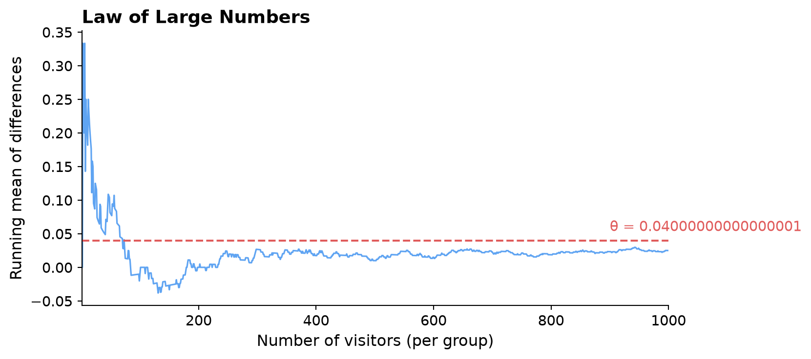
The Law of Large Numbers (LLN) tells us that as the sample size grows, the sample mean converges to the true population mean. Applied here: as we accumulate more visitors, \(\hat\pi_A \to \pi_A\) and \(\hat\pi_B \to \pi_B\), which means \(\hat\theta \to \theta\). This is the foundational guarantee that our estimator will eventually get it right — if we collect enough data.
We can visualize the LLN directly. For each visitor \(k = 1, 2, \ldots, 1{,}000\), we compute the difference between the \(k\)-th CTA A outcome and the \(k\)-th CTA B outcome, then track the cumulative average of those differences as we add one observation at a time.
Figure 1: Cumulative average of the per-visitor differences between CTA A and CTA B outcomes. The dashed line marks the true θ = 0.04.
The plot makes the LLN tangible. With only a handful of observations the running average bounces around wildly — a single sign-up swings the estimate dramatically when the denominator is small. But as we accumulate visitors the noise averages out, and the estimate settles steadily toward the true \(\theta = 0.04\). By the time we have 500 or more visitors per group, the estimate is reliably close to the truth.
Bootstrap Standard Errors
Knowing that our estimator converges to the truth is reassuring, but it doesn’t tell us how precise it is for any specific sample size. We want not just a point estimate \(\hat\theta\) but also a confidence interval that honestly communicates our uncertainty.
One elegant way to estimate the variability of any statistic is the bootstrap. Instead of deriving a formula for the standard error from first principles, we let the data speak for themselves. The idea:
Treat your observed sample as if it were the population.
Draw a new sample of the same size with replacement from it.
Compute \(\hat\theta^*\) on this “resample.”
Repeat many times and look at the spread of the resulting \(\hat\theta^*\) values.
The standard deviation of the bootstrapped estimates is our bootstrapped standard error — a data-driven measure of how much \(\hat\theta\) would vary across different samples of the same size.
The two standard error estimates are almost identical — reassuring evidence that the bootstrap is working correctly. The 95% confidence interval runs from roughly np.float64(-0.011) to np.float64(0.061). Since this interval excludes zero, we have preliminary evidence that the two CTAs are not equivalent. We will test this more formally below.
The Central Limit Theorem
The bootstrap gave us a practical way to measure uncertainty. But there is a deeper theoretical result at work: the Central Limit Theorem (CLT).
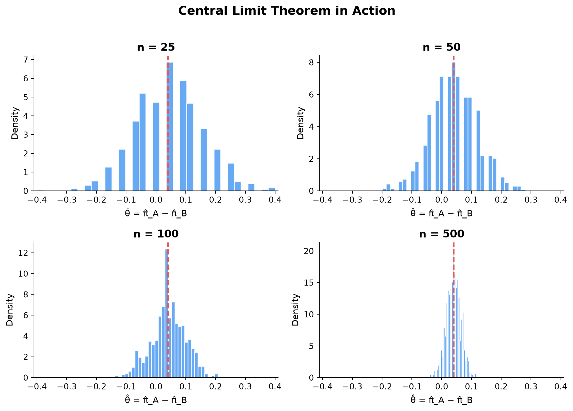
The CLT states that regardless of the shape of the underlying population distribution, the sampling distribution of the sample mean becomes approximately Normal as the sample size grows. Because \(\hat\theta = \bar{X}_A - \bar{X}_B\) is a difference of two sample means, the same result applies: for large enough samples, the distribution of \(\hat\theta\) across repeated experiments is approximately Normal, even though the underlying data are Bernoulli (just zeros and ones).
To see this in action, we run a simulation for four different sample sizes — \(n \in \{25, 50, 100, 500\}\). For each, we repeat the experiment 1,000 times and plot the distribution of \(\hat\theta\).
Figure 2: Sampling distribution of θ̂ for four sample sizes, each based on 1,000 simulated experiments. The red dashed line marks the true θ = 0.04.
At \(n = 25\) the histogram is lumpy and asymmetric — there simply aren’t enough observations for the averaging to kick in. As we move to \(n = 50\) and \(n = 100\), the bell shape becomes increasingly apparent. By \(n = 500\) the distribution is strikingly Normal and tightly centered on the true \(\theta = 0.04\). This progression is the CLT in action, and it’s the theoretical backbone for everything in the next section.
Hypothesis Testing
Now that we’ve confirmed (visually and theoretically) that the sampling distribution of \(\hat\theta\) is approximately Normal for large samples, we can use that fact to conduct a formal hypothesis test.
We frame the question as a choice between two competing claims:
Null hypothesis\(H_0\): \(\theta = 0\) — the two CTAs perform identically.
Alternative hypothesis\(H_1\): \(\theta \neq 0\) — one CTA is better than the other.
The Test Statistic
To assess whether our estimate is surprising under \(H_0\), we form the z-statistic:
\[z = \frac{\hat\theta - 0}{SE(\hat\theta)}\]
The logic step by step:
By the CLT, \(\hat\theta\) is approximately Normal for large samples. Under \(H_0\), the mean of that distribution is 0.
Dividing a Normal random variable by its standard deviation gives a standard Normal\(N(0,1)\). So under \(H_0\), \(z \;\dot\sim\; N(0,1)\).
Because we know the null distribution of \(z\), we can ask: how probable is a value at least as extreme as what we observed? That probability is the p-value.
Why Is It Sometimes Called a “t-test”?
When textbooks call this a t-test, they invoke a result from a different setting: if the raw data are Normally distributed and the variance is unknown, the standardized statistic follows an exact \(t\)-distribution. In our case the data are Bernoulli, so there’s no exact \(t\)-distribution result. The CLT gives us approximate Normality, making this more precisely a z-test. For large samples the \(t\) and \(N(0,1)\) are nearly identical, so the distinction rarely matters in practice — but it’s important to understand why.
With a p-value well below 0.05, we reject the null hypothesis. The data provide statistically significant evidence that CTA A and CTA B produce different sign-up rates.
The T-Test as a Regression
Here is something surprising: the two-sample test we just ran is mathematically identical to a simple linear regression. This connection is more than a curiosity — it shows that the OLS machinery subsumes hypothesis testing as a special case, and it points toward how to generalize beyond two groups.
The Setup
We stack the CTA A and CTA B data into a single dataset with two columns:
\(Y_i\): 1 if visitor \(i\) signed up, 0 otherwise
\(D_i\): 1 if visitor \(i\) saw CTA A, 0 if they saw CTA B
Then we fit:
\[Y_i = \beta_0 + \beta_1 D_i + \varepsilon_i\]
Interpreting the Coefficients
\(\beta_0\) is the expected value of \(Y_i\) when \(D_i = 0\) — the mean of the B group, which estimates \(\pi_B\).
\(\beta_0 + \beta_1\) is the expected value when \(D_i = 1\) — the mean of the A group, which estimates \(\pi_A\).
The coefficient estimate and test statistic match our two-sample calculation almost exactly. The standard errors differ very slightly because OLS assumes a single pooled variance, while our two-sample formula uses separate estimates for each group — a distinction that matters little when sample sizes are equal and proportions are similar.
The deeper point: once you express a comparison as a regression, you can add covariates to reduce noise, include multiple treatment arms, or model interactions between the treatment and visitor characteristics — all using the same software and the same interpretation framework.
The Problem with Peeking
Our analysis so far has been clean: collect 1,000 observations per group, then run one test. But in practice, data arrives sequentially and the temptation to peek at interim results is real. Your boss wants to know if there’s a winner after every 100 new visitors. If any peek shows significance at \(\alpha = 0.05\), she wants to stop the experiment and declare victory.
This seems harmless — after all, each individual test uses the same \(\alpha = 0.05\) threshold. But it isn’t harmless, and the simulation below shows exactly why.
The Problem
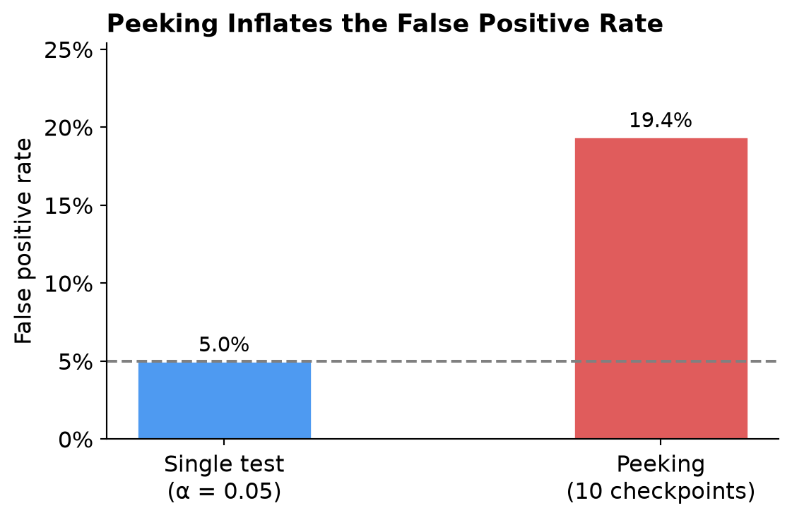
Each test at \(\alpha = 0.05\) has a 5% chance of a false positive when \(H_0\) is true. But 10 peeks mean 10 chances to get lucky. The probability that at least one of those tests produces a false significant result is far higher than 5%.
Simulation
We set up a world where \(H_0\) is true (\(\pi_A = \pi_B = 0.20\), so \(\theta = 0\)) and simulate 10,000 experiments. In each experiment we peek after every 100 visitors per group.
Figure 3: Empirical false positive rate under a peeking strategy (10 checkpoints) versus a pre-specified single test at α = 0.05.
The empirical false positive rate under peeking is approximately 19.4% — roughly 3.9× the nominal 5%. In other words, even when the two CTAs are identical, the peeking strategy would declare a winner in about 19% of experiments. You would routinely ship a change that has no real effect, simply because you looked at the data too many times.
This is not a minor technicality. It is one of the most common pitfalls in applied A/B testing. The frequentist guarantee — “if \(H_0\) is true, I will wrongly reject it only 5% of the time” — applies to a pre-specified single test, not to a repeated-peeking strategy. If you want to peek, you need methods designed for sequential testing (such as sequential probability ratio tests or alpha-spending functions) that control the false positive rate across all peeks jointly.
All simulations in this post were run in Python with a fixed random seed for reproducibility.